Train your own model with PhotonAI

Download this notebook

What is PhotonAI?#

PhotonAI

PhotonAI is a high-level Python API with which machine learning pipelines can be created quickly and easily. It is based on well-known frameworks such as Scikit-learn and Keras. The so-called hyperpipes can be used to automate the optimization of hyperparameters and other functions offer the possibility to compare or combine different methods. The Wizard also enables the generation of PhotonAI code via a web interface, making it particularly easy to get started.

For Python, PhotonAI can be installed directly in the terminal via pip:

pip install photonai

Compatibility problems#

To avoid this, it is advisable to work in a virtual environment. Python offers many options for this. We use Virtualenv or the venv module supplied since Python 3.3. One of the best-known environments is Anaconda.

Project folder and data#

Clone or copy the Git repository. Then the path to this project can be found in the folder where the repository is located. We define the path below. This must be adapted.

In our example, we have chosen a freely available data set from Kaggle, which contains data and prices for used cars (100,000 UK Used Car Data set). Download this file and enter the path to the data below. We also enter the path here. This must be adapted.

PROJECT_DIR = "<path to incubai repository>/1_1_PhotonAI/notebooks/"

DATA_DIR = "<path to data>"

Erstellung der Pipeline#

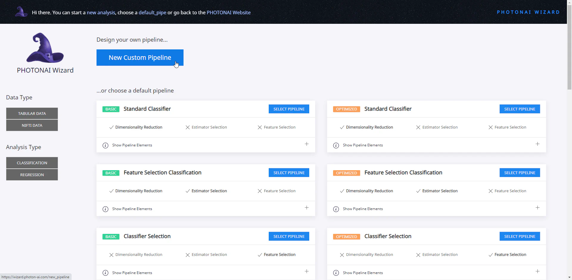
We first use the PhotonAI Wizard to create our model and design our own new pipeline there.

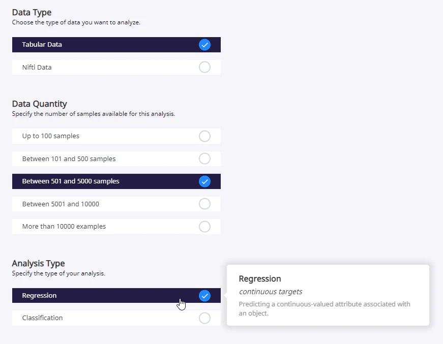
In our example, we have decided to use a freely available data set from Kaggle, which contains data and prices for used cars (100,000 UK Used Car Data set). We will limit ourselves to one car manufacturer (VW) and try to predict the price. The initial settings are directly dependent on the structure of our data set and our task. They may therefore differ for other data. However, the simplified operation of PhotonAI and the wizard in particular means that some data and tasks are not (yet) supported. For example, only tabular and Nifti data are currently available for selection in the wizard. Furthermore, it is only possible to perform a regression or classification. For other types of data or analysis, it is therefore necessary to use TensorFlow, PyTorch or similar packages.

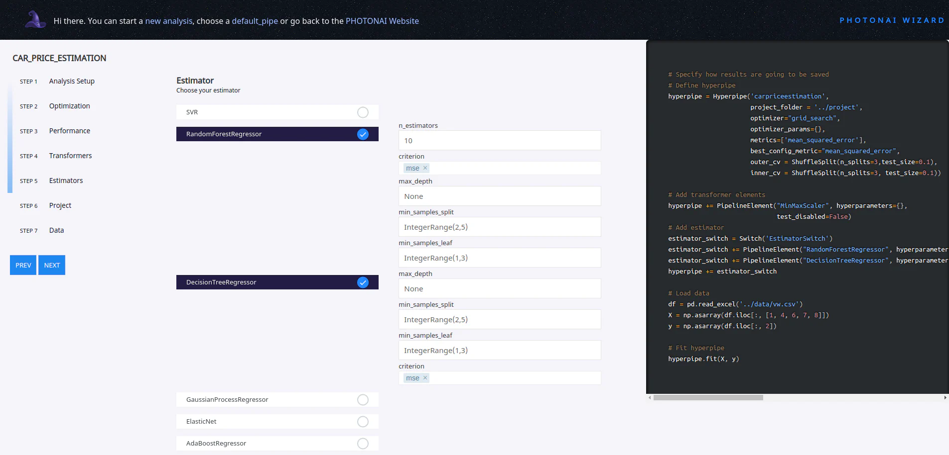
While you are making the various settings, you can view the corresponding program code live on the right-hand side. This also makes the wizard suitable for learning how to use the PhotonAI package. In our example, we add two different estimators whose performance is later automatically compared by PhotonAI.

The created code can now be downloaded. As in the following code, make sure that the structure is adhered to. For example, this Jupyter notebook is located in the app folder, which is also located together with the project folder on the same data level (1_1_PhotonAI). The project folder is used by PhotonAI as a cache for logs and models.

Customizing the pipline#

The code provided by the wizard is based on an Excel table as a data set. Therefore, in the code in the section: Load data the read_exel() must be replaced by read_csv.

Please also specify the data dir!

Training the model

The pipeline should now be ready. The following cell can be executed. During the training, we receive regular updates on the console about the performance and at the end a short summary of the best configurations that the hyperparameter search has produced.

# Beispielkonfiguration

# -------------------- GENERATED WITH PHOTON WIZARD (beta) ------------------------------
# PHOTON Project Folder: ../project

import pandas as pd
import numpy as np
from photonai.base import Hyperpipe, PipelineElement, Switch
from photonai.optimization import IntegerRange
from sklearn.model_selection import ShuffleSplit

# Specify how results are going to be saved
# Define hyperpipe
hyperpipe = Hyperpipe('carpriceestimation',
                    project_folder='../project',
                      optimizer="grid_search",
                      optimizer_params={},
                      metrics=['mean_squared_error'],
                      best_config_metric="mean_squared_error",
                      outer_cv=ShuffleSplit(n_splits=3, test_size=0.1),
                      inner_cv=ShuffleSplit(n_splits=3, test_size=0.1))

# Add transformer elements
hyperpipe += PipelineElement("MinMaxScaler", hyperparameters={},
                             test_disabled=False)
# Add estimator
estimator_switch = Switch('EstimatorSwitch')
estimator_switch += PipelineElement("RandomForestRegressor", 
                                    hyperparameters={
                                        'min_samples_split': IntegerRange(2, 5),
                                        'min_samples_leaf': IntegerRange(1, 3)
                                        },
                                    n_estimators=10, 
                                    criterion='squared_error', 
                                    max_depth=None)
estimator_switch += PipelineElement("DecisionTreeRegressor", 
                                    hyperparameters={
                                        'min_samples_split': IntegerRange(2, 5),
                                        'min_samples_leaf': IntegerRange(1, 3)
                                        },
                                    max_depth=None, 
                                    criterion='squared_error')
hyperpipe += estimator_switch

# Load data
# PLEASE UPDATE DATA DIR HERE!
df = pd.read_csv(f'{DATA_DIR}/vw.csv')
X = np.asarray(df.iloc[:, [1, 4, 6, 7, 8]])
y = np.asarray(df.iloc[:, 2])

# Fit hyperpipe
hyperpipe.fit(X, y)

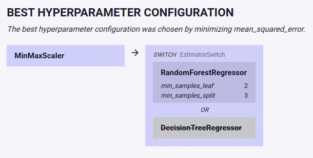
In addition, a new folder is created in +project/+, which contains some files with important information about the training run. Of course, the optimal model photon_best_model.photon and the file photon_result_file.json are particularly important here. This can be viewed with the PhotonAI Explorer. First, a summary of the complete pipeline is displayed. In our case, we can see directly that the RandomForestRegressor has performed better than the DecisionTreeRegressor.

In addition to numerous other plots, we can, for example, evaluate the performance of our model by directly comparing predicted prices and ground truth prices.

Test model#

Although the plots and metrics displayed in the Explorer are extremely helpful in evaluating our model, we still want to test our finished model again with our own inputs. To do this, we use the code below.

The file path must still be added to best_model_path. This can be found in the folder project/carpriceestimation_result.

from photonai.base import Hyperpipe

dummy_data = [[2019, 12132, 145, 42.7, 2.0]]
RESULT_DIR = "<path to result>" 
# e.g. carpriceestimation_results_2023-11-15_12-03-05

best_model_path = f'{PROJECT_DIR}/{RESULT_DIR}/best_model.photonai'

hyperpipe = Hyperpipe.load_optimum_pipe(file=best_model_path)
result = hyperpipe.predict(dummy_data)
result = hyperpipe.inverse_transform(result.reshape([1, -1]))[0][0, 0]

print(result)